Workflows
Workflow is the common name for the visual data analysis processes that are constructed in Sympathy for Data. In general, the visual workflows consist of a number of visual building blocks which are connected graphically with wires. The building blocks in Sympathy for Data are called nodes and are visual shells connected to underlying Python code that defines the functionality of the node. It is only the nodes in the workflows that perform operations on the actual data. The graphical wires represent the “transportation” of data between the nodes.
A workflow can be saved to a file, which by default will have the extension .syx. The syx-files include the graphical structure of both the workflows and any subflows as well as all the parameter settings for each node. To save a workflow click Save or Save as… in either the toolbar or in the File menu.
In Sympathy data always flows from left to right. This means that the right-most node is also the “last” node in the workflow. By double-clicking on the last node, you will start execution of any nodes to the left of that node. This might be used to execute an entire workflow (or at least everything that is connected to that node). Another way to execute an entire workflow is to simply push the “Execute” button in the toolbar.
Apart from nodes, you can also place textfields in the workflow. This is useful if you want to add a comment or description to your workflow. These text fields become a part of the workflow and are saved together with all other elements in the workflow file. To create a textfield click the button named “Insert text field” in the toolbar, then draw a rectangle on the workspace. An empty text field will appear, and by clicking in it you will be able to add some text.
Nodes
The nodes in Sympathy can be added to the workflow from the node library window, where the nodes are categorized by their functionality. Simply grab a node and drop it on the workspace.
The name of a node is located below the node. You can edit the name of a node simply by clicking on its current name. This can be used as a documentation tool to make your workflow easier to understand.
Double-clicking on a node will execute it. If other nodes need to run first your node will be queued while waiting for the other nodes. When a node is queued or executing you can right-click on it and choose Abort if you want to cancel the execution. If a node has already been executed and you want to run it again, the first thing you have to do is to reload the node, by right-clicking on it and choosing Reload. After that you can run it again.
Many nodes can be configured to perform their task in different ways. Right clicking on a node and choosing Configure will bring up the configuration GUI for that node. Some nodes have very simple configuration GUIs whereas other nodes have very complex configuration GUIs. You can read the help texts for any specific node by right clicking on a node and choosing Help.
Node states
The color of the background indicates the state of the node and in the table below the different states are presented together with their corresponding colors. Additionally there is also a special state associated with nodes executed without intermediate files, see Node states.
State |
Color |
State icon |
Explanation |
|---|---|---|---|
Armed |
Beige |
None |
The node is ready for execution. |
Error |
Red |
Warning triangle |
An error occurred during the last execution of the node. |
Disconnected |
Light gray |
None |
The node has disconnected input ports. |
Done |
Green |
Check mark |
Successfully executed. |
Queued |
Blueish gray |
Analog clock |
The node is queued for execution. |
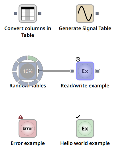
A sample of nodes in different states. The first row of nodes have not yet been executed, but while the Generate Signal Table node can the executed right now, the Convert columns in Table node is disconnected and needs input before it can be executed. The second row of nodes are being executed right now. The node to the left (Random Tables) is currently executing and Read/write example is queued and will be executed as soon as Random Tables is done. The nodes in the final row have both been executed, but while the Hello world example node was executed successfully the Error example node encountered an error during execution (as it is designed to do).
Missing Nodes
A node can also be missing in the currently loaded libraries. Such nodes will be shown as if they were in Error state and cannot be used until the library has been loaded.
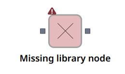
In order to find out which library that the node belongs to, the first parts of the identifier should be a good start. It is found through the node’s context menu at Advanced -> Properties -> General -> Identifier. In most cases, nodes from the same library should have the same prefix, the library identifier. Once you have determined which library is missing, add it and the node goes back to normal.
Ports
On the sides of the nodes are small symbols representing the node’s ports for incoming and outgoing data. Since the workflows are directed from left to right, the inputs are located on the left side and the outputs are on the right side.
The ports can have different symbols representing different data types. It is only possible to connect an output port with an input port of the same type. The type system in Sympathy thus ensures that only compatible nodes can be connected. See Port types for a list of different port types.
No real data is transferred between the nodes, instead paths to temporary files are exchanged. It is these temporary files on the disk that contain the actual data. Double clicking on an output port will open the data on that port in an internal data viewer.
Optional ports
Some nodes have a configurable number of ports. For example Extend List can have 2 or more input ports. To add another simply right-click on the port and choose Create. The tuple nodes are another example of a node which can get more ports in the same way.
If there are currently no port of the desired kind you instead have to right-click on the node and choose select Ports->Input->Create or Ports->Output-Create. There is a special input port called “Configuration Port” which can be added to any node. It will be covered separately. Furthermore there are 3 special ports, Output Text, Warning Text, and Output and Warnings Text. These can be used to access text output such as printed lines and warnings from ports of text type.
Added ports and some of the default ports, for example the port named Y of Fit Texts, can be removed by right-clicking on the port and selecting Delete.
Addition and removal of ports is only allowed if it does not violate the types. This should be considered when modifying ports on nodes that have ports whose type depends on other ports. For example, the output port of Tuple depends on the number of input ports.
Configuration Port
On any node you can add an optional configuration port which can be used to customize the node’s configuration using data. When added to a node it can be used to substitute parameter values in the configuration. The data connected to the configuration port can be any of a number of different types, but will most typically be either a Table or JSON.
JSON
To create JSON data you can use Create Json or Text to Json.
For example, if we wanted to customize the number of columns generated by Random Table using the configuration port and Create Json simply right-click on Random Table and choose Ports->Input->Create->Configuration Port. Then connect Create JSON and configure it in the following way:
{'column_length': {'value': 1}}
When executed the Random Table node will now produce only one row. ‘column_length’ is the name of a parameter, if the parameters are nested in groups, the JSON configuration also needs to be nested. Luckily, few nodes use nested parameters. If Random Table had nested its ‘column_length’ parameter in a group called ‘all_parameters’ you would type:
{'all_parameters': {'column_length': {'value': 1}}}
to get the same effect as in the flat case.
For normal scalar parameters it is ‘value’ that needs to be changed, but for list parameters it is often best to change ‘value_names’. For example, to configure the selection used by Select Columns in Table:
{'columns': {'value_names': ['0', '1']}}
When executed would select columns named ‘0’ or ‘1’.
Then what is the parameter structure of some node? Create the node and right-click, choose Advanced->Properties and the select the Parameters Tab. “Parameter Model” displays the relevant information (and more).
Using the json structure, it is possible to set the value of several parameters (even all of them) at once by providing values for several keys.
Finally there is also the possiblity for a node to output its configuration on a port. To get configuration output, simply add the output version of the Configuration Port. This can be useful in allowing the configuration from one node to control other nodes or to make it easier to modify specific parts using other nodes.
Data Binding
Data bindings are available for nodes that have a input Configuration Port and makes it possible to configure how the configuration data should be applied to the configuration parameters. The data binding has two modes of operation, one for JSON type configuration data and one for other configuration data (typically table data). The configuration of the data binding is shown as a separate tab next to the normal configuration and indicates that the normal configuration data may be replaced completely or to some extent.
With JSON configuration, the data is applied to all configuration parameters (see JSON). The data binding allows selecting a dictionary key to treat as the data root. This makes it possible to pass several node configurations in the same JSON data and select which part that should apply for each node. The root is used by default.
With table configurable data, data bindings are applied to individual configuration parameters.
When Advanced development options are enabled in General, it is possible to hide the Data Binding tab, by right-clicking on the tab and unchecking Show (check to show them again). The tab will become disabled and will be completely hidden to any user without Advanced development options enabled. This option can be used to hide implementation details from normal users of your flow, but note that it can be confusing if the behavior does not match the configuration as shown in the node configuration that they see.
Connections
Creating connections
The connections are represented by wires between the nodes and are established by drag and drop. Click on an output port and drag to a free input port on another node or vice versa. Connecting several connections to the same input port is not possible.
It is also possible to auto-connect ports by holding down the Shift modifier key on your keyboard while moving a node. A transient connection will be shown between the two closest ports which the same port type if the ports are not too far apart. To materialize the connection one just releases the mouse button.
To connect the node in focus to several ports in the auto-connect mode, one can use the c key while the transient connection is shown. This will create the connection and pick the next fitting port pair if available for the selected node. Should no transient connection be shown, move the selected node closer to the node you want to connect to.
To exit the auto-connection mode without making connection either release the modifier key, press the Esc key or move the selected node to a region far enough away so no transient connection is shown.
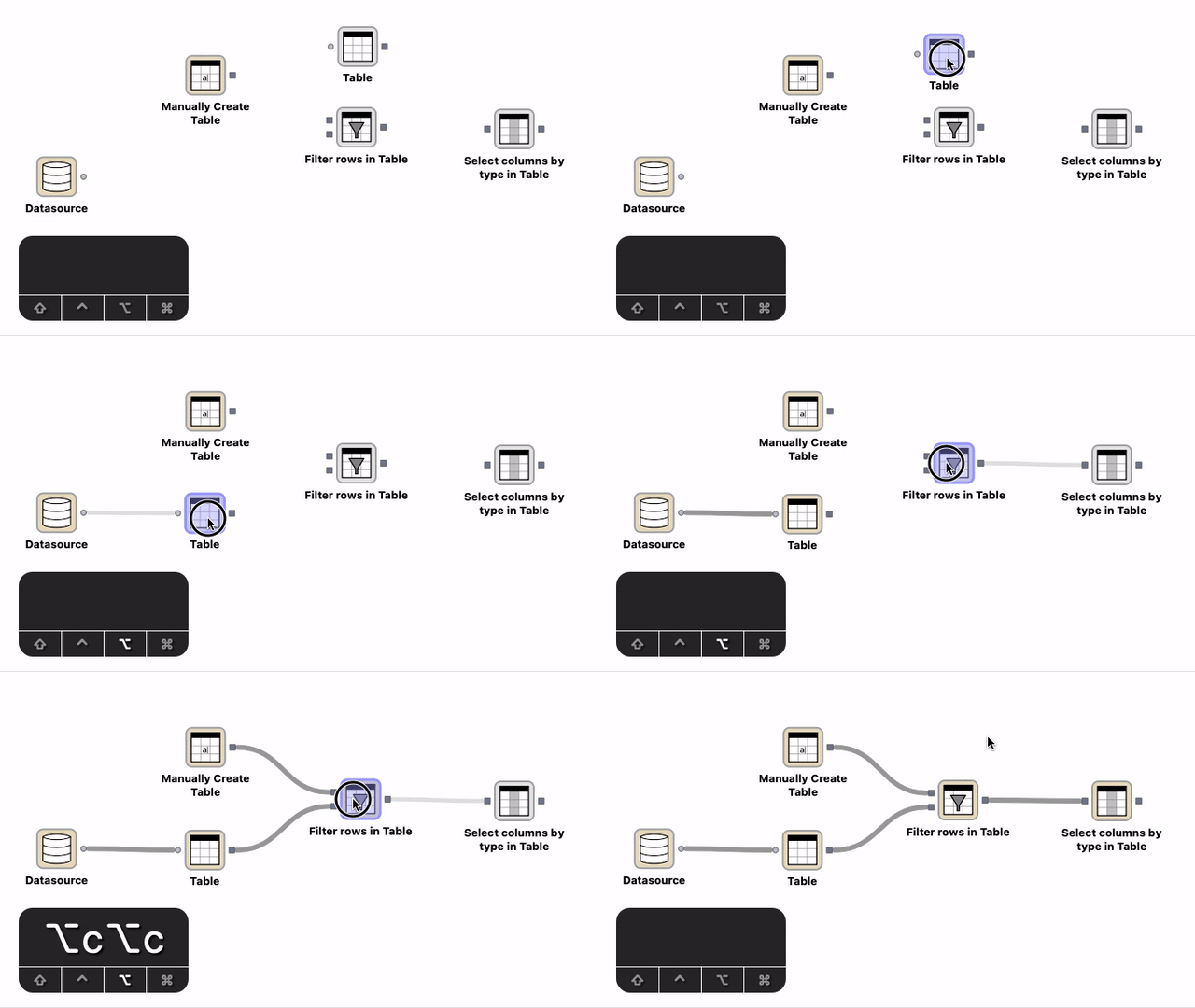
Creation of connections with the help of the auto-connect functionality. Select a node, press the Shift modifier key and move the node close to the other node you want to connect to. A transient connection appears to the closest port. Create the connection by either releasing the mouse button or pressing c.
Deleting connections
The nodes can be disconnected by right clicking the wire and choosing Delete or by selecting the connection and pressing Delete on your keyboard. In addition to using the keyboard shortcut, mouse right-click will popup a context menu which allows connections to be removed.
Route points
Route points can be a helpful element to improve the readability of a workflow and can be moved around. They can be created either by double-clicking on an existing connection or with the help of the connection’s context menu.
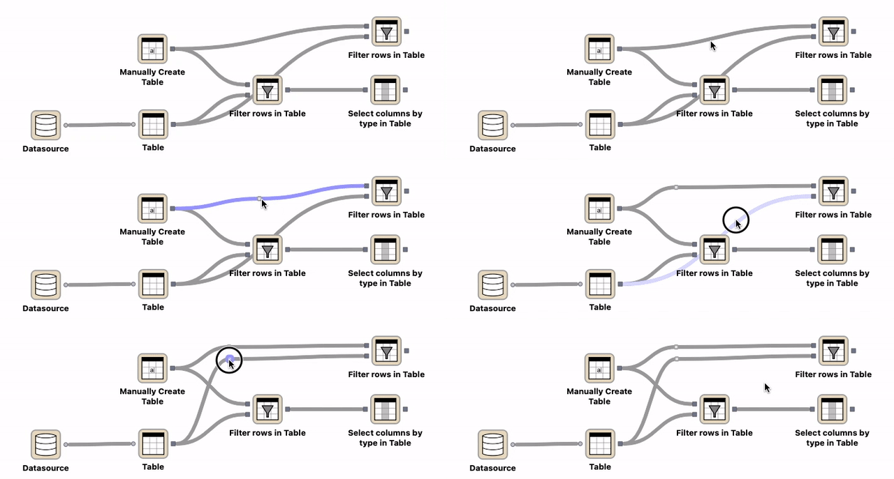
Double-click on an existing connection which creates a new route point. Move the route point to the desired location.
Text fields
Text fields are a kind of comments or annotations that you can add to your flow. They are purely cosmetic and thus do not in any way affect the execution of a flow. But they can be a great way to add some documentation to a flow.
To add a text field use the Insert text field button in the toolbar. To edit the text in a text field, simply double-click on it and an editor will appear. In the context menu you can also change the background color of the text field. Markdown syntax is supported in text fields.
