Debugging nodes
Debugging nodes using Spyder
Warning
Spyder based debugging is only available when the Spyder plugin is installed and available in your python environment. This might the be case when using some Windows installers for Sympathy.
When a node is not working as expected a very handy tool to use is the node debugger. Run a workflow up and to the node that you want to debug. Right-click the node and choose “Debug” from the context menu.
This will bring up Spyder with the node with correct data on the input ports,
ready to be debugged simply by selecting the file and pressing Run
file. After running the code at least once you will also have access to the
node’s node_context in the interactive python prompt under the name dnc
(short for debug node context). For example, dnc.output[0] will show the
data on the first output port, if there is any. See Node context reference for
information on how to use the dnc variable.
Alternatively, more fine grained line and break-point based debugging can also be used. Place a break-point on a line in the execute function of the node you have selected for debugging and press Debug file (Ctrl+F5). Now, wait until execution stops on a line and continue by pressing Continue execution until execution finally stops on the line with the break-point. In addition to the execute function, break-points can be placed on any line of code that is called by the execute function, this provides even more detailed control and is helpful when debugging F(x) scripts. To debug F(x) scripts, debug the F(x) node (node_fx_selector.py) and then place the break-point in the execute method of your script file. Finally, make sure that the file node_fx_selector.py is the active file in spyder and press Debug file.
Note
There are some limitations when using Spyder based debugging in Sympathy. Only execute methods can be debugged and it can happen that the console ends up in a bad state where debugging cannot proceed. When you have problems getting debugging to work, make sure that the current file is the one containing the node that you want to debug and close all consoles to make sure that you get a new fresh console before retrying.
Please refer to the Spyder manual for more info on it’s debugging features.
Debugging nodes using PyCharm
PyCharm is an external IDE (not included in Sympathy) which provides good debugging support for Symapthy.
In order to debug Sympathy in PyCharm follow these steps.
Create a new Project
Choose the Python interpreter (python.exe) used to run Sympathy as the Project Interpreter. You may have to wait some time for indexing to complete.
In Settings->Project->Project Structure, add the folders containing the code that you want to debug using Add Content Root. For example, in order to debug anything from Sympathy itself (including the standard library nodes) add <Python>/Lib/site-packages/sympathy and <Python>/Lib/site-packages/sylib. Then you may have to wait for another indexing.
In Run->Edit Configurations, create a new configuration that uses the Project Interpreter. Choose a name that is easy to remember. Set Script: sympathy/__main__.py, and Script parameters: gui.
In Run, choose Debug ‘<your-configuration-name>’, this will start Sympathy in debug mode. When debugging you can set breakpoints by clicking on the left margin. When execution in debug mode reaches a breakpoint, it will stop there and allow you to interact with it.
Profiling nodes and workflows
If your node or workflow is running too slow you can run the profiler on it to see what parts are taking the most time. If you have configured Graphviz, see Configuring Graphviz, you will also get a call graph.
To profile a single node simply right-click on a node that can be executed and choose Advanced->Profile. This will execute the node and any nodes before it that need to be executed, but only the node for which you chose Profile will be included in the profiling. To profile an entire workflow go to the Controls menu and choose Profile flow. This will execute all nodes in the workflow just as via the Execute flow command. After either execution a report of the profiling is presented in the Messages view. Profiling of single subflows is similar to profiling of single nodes but include all the executable nodes in the subflow.
The profile report consists of a part called Profile report files and a part called Profile report summary.
Profile report files
The Profile report files part of the profile report consists of two or four file paths. There is always a path to a txt file and a stats file, and also two pdf files if Graphviz is configured, see Configuring Graphviz. The txt file is a more verbose version of the summary but with full path names and without any limit on the number of rows. The first pdf file contains a visualization of the information in the summary, also called a call graph, and the second a call graph of flows and nodes.
The function call graph contains a node for each function that has been called in the profiled code. The color of the node gives you a hint about how much of the total time was spent inside a specific function. Blue nodes represent functions with low total running time and red nodes represent functions with high total running time. The nodes have the following layout:
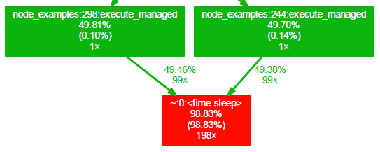
First row is the name of the function. Second row is the percentage of the running time spent in this function and all its children. Third row (in parentheses) is the percentage of the running time spent in this function alone. The forth row is the total number of times this function was called (including recursive calls).
The edges of the graph represent the calls between functions and the label at an edge tells you the percentage of the running time transferred from the children to this parent (if available). The second row of the label tells you the number of calls the parent function called the children.
Please note that the total running time of a function has to exceed a certain cut-off to be added to the call graph. So some very fast workflows can produce almost empty call graphs.
A third file will also always be provided with the file ending “.stats”. This file contains all the statistics that was used to create the summary and the call graph. To begin digging through this file open a Python interpreter and write:
>>> import pstats
>>> s = pstats.Stats('/path/to/file.stats')
>>> s.print_stats()
For more information look at the documentation for the Stats class.
Profile report summary
The summary contains a row for each function that has been called in the profiled code. Several calls to the same function are gathered into a single row. The first column tells you the number of times a function has been called. The next four columns measure the time that it took to run a specific function. In the last column you can see what function the row is about. See https://docs.python.org/2/library/profile.html for details on how to interpret this table.
The summary also includes up to 10 node names from nodes included in the profiling and an indication of the number of nodes that were ommited to save space.
Configuring Graphviz
For the call graph file to be generated Graphviz will have to be installed and the path to the bin folder which contains dot will have to be in either PATH or Graphviz install path, see Debug Preferences.
Writing tests for your nodes
As with any other code, writing tests for your nodes is a good way of assuring that the nodes work and continue to work as you expect.
Test workflows
The easiest way to test the execution of your nodes is to add them to a workflow (.syx) and put that workflow in the test flows folder. See Libraries for information about where to put test flows in your library.
In some cases it can be enough to test that the flows can execute without producing exceptions or errors, in other cases, the actual data produced need to be checked. For comparing data, Conditional error/warning and Assert Equal Table may come in handy.
Unit tests
It is also a good idea to write unit tests to ensure the quality of your
modules. Put unit tests in test.py. See Libraries for information about
where test.py is located. You can also create new files next to test.py with
names matching test_*.py and put the unit tests there. If the tests are named
correctly they can be run automatically by the Python module nose (or
pytest). See https://nose.readthedocs.org/en/latest/finding_tests.html for
more details about how to name your unit tests. Cd into the library directory and
run nosetests to run all unit tests there.
For example a unit test script that tests the two functions foo() and
bar() in the module boblib.bobutils could be called
test_bobutils.py and look something like this:
import numpy as np
from nose.tools import assert_raises

import boblib.bobutils


def test_foo():
    """Test bobutils.foo."""
    assert boblib.bobutils.foo(1) == 2
    assert boblib.bobutils.foo(0) == None
    with assert_raises(ValueError):
        boblib.bobutils.foo(-1)


def test_bar():
    """Test bobutils.bar."""
    input = np.array([True, False, True])
    expected = np.array([False, False, True])
    output = boblib.bobutils.bar(input)
    assert all(output == expected)
For more examples of real unit tests take a look at the documentation for the
nose module at https://nose.readthedocs.org/.
You can run only the unit tests of your own library by running the following command from a terminal or command prompt:
# Assuming nodes is installed.
# Otherwise, pip install nose.
nosetests <library path>