Machine Learning Concepts

Machine learning is a method of data analysis that builds analytical models based on empirical data. This models can be used for gaining insight into the data, performing predictions or simply for transforming the data. Scikit-learn is a large Open Source framework of machine learning algorithms that are included in Sympathy for Data together with nodes and functions for accessing scikit learn or adding upon available algorithms.

When working with machine learning in Sympathy a core datatype is the model object. These objects represent both the algorithms and the internal data created by the algorithms which are used for machine learning. The source nodes of these types of models typically do not directly perform any calculation on the data, which is rather done when the models are applied to some dataset.

For example, if you start with a “Decision Tree Classifier” node and run it, then you get an unfitted model object. By connecting the model to a Fit node (uppermost port), and giving some example X (middle port) and Y (bottom port) data, then you can “train” the model from X. In the screenshot below the “Example dataset” node has been configured to use the “Iris” dataset. On the right side we can see the output model created by the Fit node. This displays the learned decision tree. This visualization requires that Graphviz/dot is installed and configured.

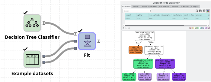
After fitting (a.k.a. training) a model you can use it to, for example, do predictions on data. This data must have the same columns as the original X data, and will produce a table with the same columns as the original Y data.

Pre-processing data

In addition to models that can perform predictions of data it is also possible to use models that do other operations such as preprocessing the input data. Examples of such nodes include the “Standard scaler” which removes the mean of the data and rescales the data to have a unit standard deviation. In order to use models of this type you typically want to use the “Fit transform” to let the model “learn” what the rescaling parameters should be and to output the transformed data.

If you later want to perform the same transformation on another dataset you can use the “transform” node with model coming as an output from the earlier fit and transform. For example, in the flow below the mean of each column in A will be subtracted from the corresponding columns in B. Note that the order of the columns and not only their names matter when applying a node.

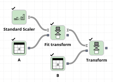
Note that you could have used a Fit node instead of Fit Transform here for the same result since the rescaled version of A is not used here.

In a real application the model given by fitting or training A would typically be exported to disk using the “Export model” node, and imported back in another flow when using it for transforming or predicting on the B dataset.

Varying number of parameters

Depending on the types of models that are used the Fit node can take either one (X) or two (X, Y) tables with inputs. Since the X-Y case is the most common, this is the default, and if you want to pass only one input (eg. when fitting a preprocessing node) you can right click on the Y port and select Delete.

Other nodes that can take a varying number of parameters are the pipeline and voting classifier nodes. In order to add more inputs to these you can right click on the node and select Ports->Input->Create. This way of adding/removing input ports works also on some other nodes in Sympathy, test for instance the tuple or zip nodes.

Pipelines

In a typical machine learning application one often needs to perform multiple pre-processing steps on the data before it is given to a machine learning algorithm for training or prediction. To simplify multiple pre-processing steps a complex pipeline model can be created out of simpler models.

These pipeline models give the data to each constituent model one at a time and transforms it before passing to the next model. When performing a training or prediction task, the last model performs the actual training or predictions.

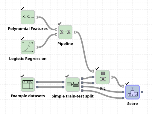
In the example above a “Polynomial features” node is used to create all polynomials of degree two from the features in the Iris dataset. These new features include, for example, petal width * petal height, petal width^2, etc. By pipelining this polynomial feature node to the logistic regression node we can improve the final output score from circa 95% to 100%.

Note that in the example above we do not use the same data to train the model and to score it. The node “Simple train-test split” splits the X and Y data into 75% that are used for training (top two output ports) and 25% that are used for evaluating how well the model learned the data (bottom two output ports).

This is only one example of how datasets can be used when evaluating models, for more advanced methods use the cross-validation nodes. You should also avoid leaking information from the test set into your choice of parameters by further splitting the data which is used during development and during final evaluation.

Machine learning examples

Many more algorithms and concepts from machine learning have been integrated with Sympathy, for more examples make sure to open the examples that are included with the Sympathy release. You can find the examples folder under the install path of Sympathy.

Examples of concepts that are covered by these examples:

• Integration with the image processing parts of Sympathy
• Face recognition of politicians using the eigenfaces method
• Training multiple times using different “hyper parameters” to find the configurations that are best for a given problem
• Using cross-validation when learning hyper-parameters
• Combining ensembles of simple classifiers for more robust classifications
• Operating on text data using the bag-of-words method
• Analyzing the quality of the trained model using ROC (receiver-operating characteristic) curves, confusion matrices, and other metrics
• Using clustering algorithms as preprocessing steps for supervised learning algorithms