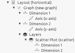
Creating New Layers
The reporting tool is based on a concept where complicated plots can be constructed from relatively simple specialized layers. Layers are put on top of each other to produce a total richer content.
Layers are rendered using a given backend. Currently there is only a backend based on Matplotlib available.
Writing New Layers
Writing new layers can be a difficult process depending on the knowledge of the details of the underlying backend. A layer is responsible for creating and updating elements which should be added to its parent graph. The reporting tool has a data binding system which should be utilized to update layer properties properly.
In the standard library of Sympathy for Data below
Library/Common/sylib/report/backends there are two folders, one for
layers and one for systems (backends). For each layer there should be an
ordinary __init__.py file, one layer.py containing miscellaneous
definitions and renderer_{backend}.py where renderer_mpl.py is the
renderer for the layer for the mpl (Matplotlib) backend.
Any new icons used must be added to the folder report/svg_icons and later
added to report/icons.py.
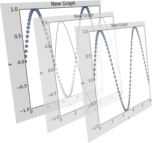
Tour of Scatter Layer
The scatter layer is a common plot type where graphical symbols represent a
coordinate pair in a two dimensional space. Its basic definition is based on
layer.py. The definition contains two dictionaries within a class;
meta and property_definitions. The first definition of meta data
below defines the visual icon of the layer, its label and default property
data. The number of items in data specifies the number of dimensions of
the layer, in this case two dimensions. To create your own two
dimensional layer it is safe to copy this structure and replace icon, label
and type with your own values.
meta = {
    'icon': icons.SvgIcon.scatter,  # Shown in toolbar
    'label': 'Scatter Plot',        # Can be seen in tree
    'default-data': {
        'type': 'scatter',          # Internal identifier
        'data': [                   # Appears in tree as dimension 1 and
            {                       # dimension 2 below Scatter Plot.
                'source': '',
                'axis': ''
            },
            {
                'source': '',
                'axis': ''
            }
        ]
    }
}
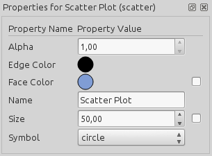
The next block called property_definitions defines all properties which can
be modified by the user. The code which takes care of changes is implemented in
the renderer, i.e. renderer_mpl.py for Matplotlib. For the scatter plot
example we have six different properties defined: name, symbol,
size, face-color, edge-color and alpha. Each property is
defined by a dictionary whose fields depend on the type of data it contains.
All properties require four fields: type, label, icon and
default.
The currently allowed values for the type field giving property editors
specialized for each type are:
- string
- integer
- float
- color
- boolean
- list
- datasource
- colorscale
- image
The label is a free text label shown to the left of the editor in the
property editor as seen in the picture below.
The icon field is a special icon for the given property. It is currently
not having any effect.
The default value of the property editor is given in default. Any new
property editor without any previous value is given the default value.
For lists an extra field called options must be given which contains a
list of available choices. The default field must contain a value equal
to one of the options.
For numeric types like integer and float there is a field called range
which defines the behavior of the
Qt spin box in the property editor.
The range field is a dictionary with three fields called min (minimum
allowed value), max (maximum allowed value)
and step (step size when clicking arrow buttons).
For some numeric and color values it is possible to bind a data source. The
binding behavior is not automatic since it must be implemented in the
renderer of the layer. The complexity of implementing a binding differs
depending on the plotting framework used for the backend. To indicate that a
property is possible to bind to a data source a field called
scale_bindable should be set to true.
The entire code for a scatter plot definition in layer.py becomes:
from sylib.report import layers
from sylib.report import icons


class Layer(layers.Layer):
    """
    ScatterLayer
    """
    meta = {
        'icon': icons.SvgIcon.scatter,
        'label': 'Scatter Plot',
        'default-data': {
            'type': 'scatter',
            'data': [
                {
                    'source': '',
                    'axis': ''
                },
                {
                    'source': '',
                    'axis': ''
                }
            ]
        }
    }
    property_definitions = {
        'name': {'type': 'string',
                 'label': 'Name',
                 'icon': icons.SvgIcon.blank,
                 'default': 'Scatter Plot'},

        'symbol': {'type': 'list',
                   'label': 'Symbol',
                   'icon': icons.SvgIcon.blank,
                   'options': ('point', 'circle', 'square'),
                   'default': 'circle'},

        'size': {'type': 'float',
                 'label': 'Size',
                 'icon': icons.SvgIcon.blank,
                 'scale_bindable': True,
                 'range': {'min': 10, 'max': 1000, 'step': 25},
                 'default': 50.0},

        'face-color': {'type': 'color',
                       'label': 'Face Color',
                       'icon': icons.SvgIcon.blank,
                       'scale_bindable': True,
                       'default': '#809dd5'},

        'edge-color': {'type': 'color',
                       'label': 'Edge Color',
                       'icon': icons.SvgIcon.blank,
                       'default': '#000000'},

        'alpha': {'type': 'float',
                  'label': 'Alpha',
                  'range': {'min': 0.0, 'max': 1.0, 'step': 0.1},
                  'icon': icons.SvgIcon.blank,
                  'default': 1.0}
    }
To implement a Matplotlib renderer for the scatter layer we have to write
some code. The file should be called renderer_mpl.py. First we need some
definitions.
import functools
from sylib.report import plugins
from sylib.report import editor_type
mpl_backend = plugins.get_backend('mpl') # get backend for matplotlib


# Mapping between symbol name to symbol used in MPL.
SYMBOL_NAME_TO_SYMBOL = {
    'point':  '.',
    'circle': 'o',
    'square': 's'
}
SYMBOL_TO_MARKER_NAME = {v: k for k, v in SYMBOL_NAME_TO_SYMBOL.iteritems()}


def create_layer(binding_context, parameters):
    """
    Build layer for MPL and bind properties using binding context.
    :param binding_context: Binding context.
        :param parameters: Dictionary containing:
                           'layer_model': a models.GraphLayer instance,
                           'axes': the MPL-axes to add layer to,
                           'canvas': current canvas (Qt-widget) we are rendering to,
                           'z_order': Z-order of layer.
        """
A common pattern is to bundle parameters which are often used in callback functions to make code shorter.
context = {
    'binding_context': binding_context,
    'path_collection': None,
    'layer_model': parameters['layer_model'],
    'axes': parameters['axes'],
    'canvas': parameters['canvas'],
    'z_order': parameters['z_order'],
    'properties': [],
    'drawing': False
}
Depending on the plotting framework different strategies needs to be developed to handle any property or data updates properly. The strategy might have to differ between different plot types within the same framework since plots can behave very different. Here we are using a single callback for updating data which takes the context as its first argument and ignoring the value sent.
There are two ways to update an MPL-plot. Either rebuild everything from scratch or only update the specific objects involved. The latter method generally gives quicker response but might be difficult to get to work properly. For cases when the plotting framework does not want to do what you expect a good fallback solution is to redraw everything. How to do this is shown later in this text.
def update_data(context_, _):
    properties_ = context_['layer_model'].properties_as_dict()
    # Remove old path collection first.
    if context_['path_collection'] is not None:
        context_['path_collection'].remove()
        context_['path_collection'] = None
For convenience there is a method in the layer data model (defined in
models.py) which extracts all data and data properties for you.
Matplotlib gives errors when the length of data in x and y does not match so
we cannot do anything until those lengths match and are not zero.
(x_data_, y_data_), _ = \
    context_['layer_model'].extract_data_and_properties()
if len(x_data_) != len(y_data_) or len(x_data_) == 0:
    return
Next we extract all property values needed to be able to generate the plot.
Some of the values need to be scaled and we are using a function from the
backend to help perform those calculations. Such utility functions are
specific to each backend since each plotting framework needs to be treated
differently. If no scale is present the scale function only returns the
scalar value. For edge-color we did not activate any data binding so we
could have omitted the scale function, but in this case it does not make any
difference. The alternative is to fetch the property value directly as done
for marker.
scale = functools.partial(mpl_backend.calculate_scaled_value,
                          context_['layer_model'])
size = scale(properties_['size'])
face_color = scale(properties_['face-color'])
edge_color = scale(properties_['edge-color'])
alpha = scale(properties_['alpha'])
marker = properties_['symbol'].get()
Here we just generate a scatter plot and store the resulting objects such that we can remove them later on. For Matplotlib we have focused on using existing plotting routines as far as possible. If performance is to be optimized it is probably more efficient to write each plotting routine from scratch using low level components of Matplotlib.
context_['path_collection'] = context_['axes'].scatter(
    x_data_, y_data_, s=size, c=face_color, alpha=alpha,
    marker=SYMBOL_NAME_TO_SYMBOL.get(marker, 'o'),
    edgecolors=edge_color,
    zorder=context_['z_order'])
Using draw_idle postpones rendering until the event loop is free. This
gives better responsibility of the GUI.
context_['canvas'].draw_idle()
Back to the code running before the callback is called. First we have to extract data and data source properties and perform the initial rendering of the plot.
(x_data, y_data), data_source_properties = context[
    'layer_model'].extract_data_and_properties()

if len(x_data) != len(y_data) and len(x_data) == 0:
    update_data(context, None)
The reporting framework contains a simple data binding system which
automatically calls callbacks of bound targets such that necessary actions can
take place on write. Wrapping and binding properties is so common that we
implemented a utility function for this in the backend for matplotlib. The
following code makes sure that the update_data callback gets called each
time the data source is changed.
if data_source_properties is not None:
    mpl_backend.wrap_and_bind(binding_context,
                              parameters['canvas'],
                              data_source_properties[0],
                              data_source_properties[0].get,
                              functools.partial(update_data, context))
    mpl_backend.wrap_and_bind(binding_context,
                              parameters['canvas'],
                              data_source_properties[1],
                              data_source_properties[1].get,
                              functools.partial(update_data, context))
In order to have the axes updated properly we add a tag to the property editor to force an entire rebuild of the plots.
# This is used to force update of axis range.
data_source_properties[0].editor.tags.add(
    editor_type.EditorTags.force_rebuild_after_edit)
data_source_properties[1].editor.tags.add(
    editor_type.EditorTags.force_rebuild_after_edit)
And for the rest of the properties we only need to call update_data on
any changes.
# Bind stuff.
properties = parameters['layer_model'].properties_as_dict()

for property_name in ('symbol', 'size', 'face-color', 'edge-color',
                      'alpha'):
    mpl_backend.wrap_and_bind(binding_context,
                              parameters['canvas'],
                              properties[property_name],
                              properties[property_name].get,
                              functools.partial(update_data, context))
To learn more about how layers can be implemented you are encouraged to study all renderers of layers and the backend code.